
Introduction
In this article, we look at the process of improving ‘Flow’ through the lens of a theorem known as Little’s Law. Think of this article as a “Little’s Law for Dummies” where we discuss:
⏳Little’s Law
🧑🏫Little’s Law Formula
🌊Little’s Law and ‘Flow’
🍕Little’s Law Example
📈Little’s Law in Project Management
⏳Little’s Law
Let’s turn the clocks back and head to the 1950s. John Little, a professor at the Massachusetts Institute of Technology (MIT), conceptualizes “Little’s Law”. Simply put, Little’s Law states that “under steady-state conditions, the average number of items in a queuing system equals the average rate at which items arrive multiplied by the average time that an item spends in the system”.
Little’s Law originally dealt with the estimation and optimization of queuing systems. However, today we see a broad range of applications of little’s law in operations management and project management amongst other fields.

🧑🏫Little’s Law Formula
So, how does Little’s Law work in practice? To answer this question, let’s have a look at Little’s Law formula:
L = λ x W
- L is the work in progress (WIP), or the items in the queuing system. Also known as inventory.
- λ is the throughput or the rate at which items arrive and leave the queuing system. Also, known as flow rate.
- W is the lead time or the average time an item spends in the system. Also known as cycle time or flow time.
The formula is also expressed as Work in progress (WIP) = Throughput x Lead time
🌊Little’s Law and ‘Flow’
So, what implications does Little’s Law have for ‘Flow’? There are two main implications.
The first implication has to do with assessing the impact of each variable. With inventory, flow rate, and flow time, we have 3 key measures that can tell us a lot about the efficiency and effectiveness of a process. What’s interesting about the relationship between these measures is that while we can change two of these measures, the third will stay constant. Thereby, we can easily measure how changing one measure can impact another. For example, if we keep the throughput constant but change the WIP, we can observe how it directly affects the flow time.
The second implication is estimating the third measure if we only know two but cannot observe the third. For instance, we may easily observe the inventory and throughput but not the flow time. With Little’s Law, we can easily calculate the flow time using the other two measures. Thereby, Little’s Law formula can also be represented as:
- Little’s Law WIP calculation: Work in progress (WIP) = Throughput x Lead time
- Little’s Law cycle time/flow time/lead time calculation: Lead time = WIP / Throughput
- Little’s Law flow rate/throughput calculation: Throughput = WIP / Lead time
🍕Little’s Law Example
As an example, let’s look at a pizza shop:
🍕On average, the pizza shop can serve 10 customers per hour (throughput).
🍕Each customer takes 30 minutes from order to complete their meal and leave the restaurant (lead time).
🍕We know that Work in progress (WIP) = Throughput x Lead time.
🍕Therefore, we can calculate the average number of customers inside the restaurant at any given time: 10 customers per hour x 0.5 hours = 5 customers (=WIP)
Additionally, the pizza shop can also make sound decisions for desired changes. For instance, if the pizza shop begins to experience an increase in demand, then it would need to identify a way to increase its throughput, but without increasing the Lead time (30 minutes) for each customer.
How could it do that? Here’s where Little’s Law can help again:
🍕We know that Throughput = WIP / Lead time.
If the restaurant wants to receive twice as many customers in the restaurant (10 customers instead of 5), and the throughput stays at the same level (10 customers per hour), it can be expected that the lead time for each customer will double from 0,5 hours to 1 hour.
🍕To prevent the lead time for the customer doubles, the pizza shop needs to increase its throughput, for example by hiring more kitchen staff or investing in bigger pizza ovens or automated equipment that allow more pizzas to be cooked at the same time.
🍕Alternatively, to prevent many customers from entering the Pizza restaurant, it could also lower the WIP by providing discounts on takeaway orders.
📈Little’s Law in Project Management
With such significant implications, Little’s Law also finds applications in project management, multi-project and portfolio management, and Kanban methodologies. In Kanban, Little’s Law is instrumental as the main focus of Kanban is to reduce the WIP. The reason for this is that doing so enables a predictable Kanban system, with lower WIP making it easier to meet deadlines. With Little’s Law, the throughput, lead time, and WIP can be calculated, thereby enabling an efficient Kanban system.
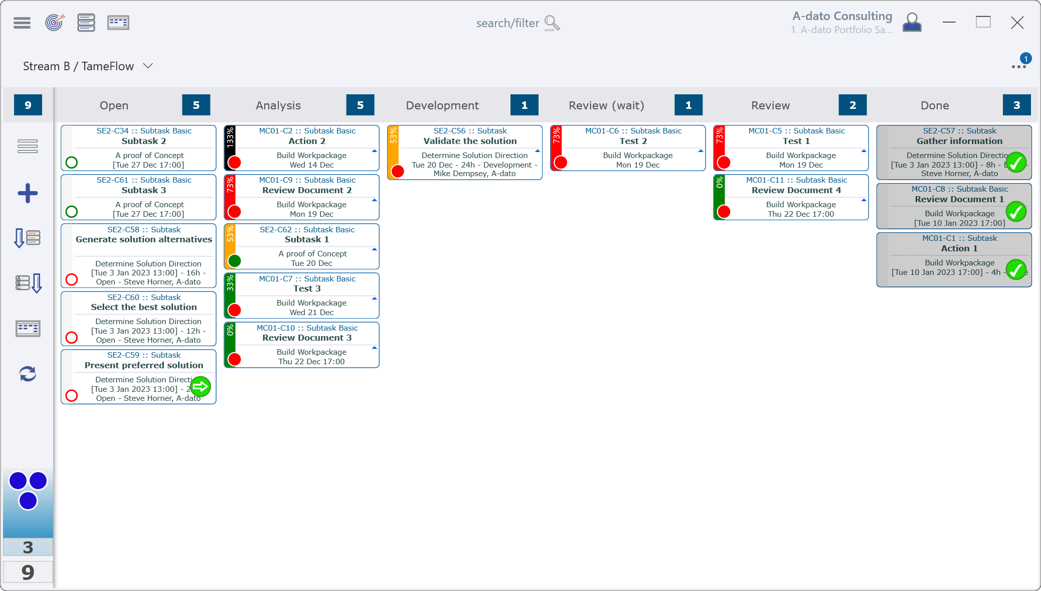
This is demonstrated in the LYNX TameFlow software which uses a Kanban board to enable the completion of projects in time while controlling your WIP. However, unlike the typical Kanban board, LYNX Tameflow can utilize buffers that enable better prioritization of tasks. The colors on the cards indicate the level of priority of a task and tell you what you need to do first before starting any new tasks. In controlling the WIP, LYNX TameFlow helps you increase throughput, thereby improving ‘Flow’.
Interested in knowing more? Click here to try LYNX TameFlow out!
References
https://link.springer.com/chapter/10.1007/978-0-387-73699-0_5
https://www.coursera.org/lecture/wharton-operations/littles-law-kyo5e
https://www.academia.edu/download/45845550/s0377-2217_2899_2900155-120160521-8368-1a5dpew.pdf
1 Comment. Leave new
very informative articles or reviews at this time.